RL Intro and Fundamentals
The code associated with this blog post can be found here.
Table of Contents
Background
In this post, I will be talking about Markov Decision Processes (MDPs), their role in reinforcement learning, and a few ways in which they can be solved. This post will first talk about methods for solving MDPs exactly, including value iteration and policy iteration. We will then discuss the reinforcement learning problem, where we assume MDPs are the underlying mechanic in our observations, but we are blind to the MDP’s reward and state transition mechanics. This will require us to infer value estimates using observation tuples and an algorithm called Q-learning.
MDPs
Formally, a Markov decision process is defined as a tuple of four things:
\[(S, A, R, T)\]$S$ is a set of states and $A$ is a set of actions available at each state. $R(s,a,s’)$ is a reward function, namely, “if I take action $a$ in state $s$ and end in state $s’$, what reward will I receive?”. Finally, $T(s,a,s’)$ is a state-transition function that defines transition probabilities between states $s$ and $s’$, given an action $a$. Solving an MDP involves maximizing the reward we can receive from the environment within a finite-time horizon.
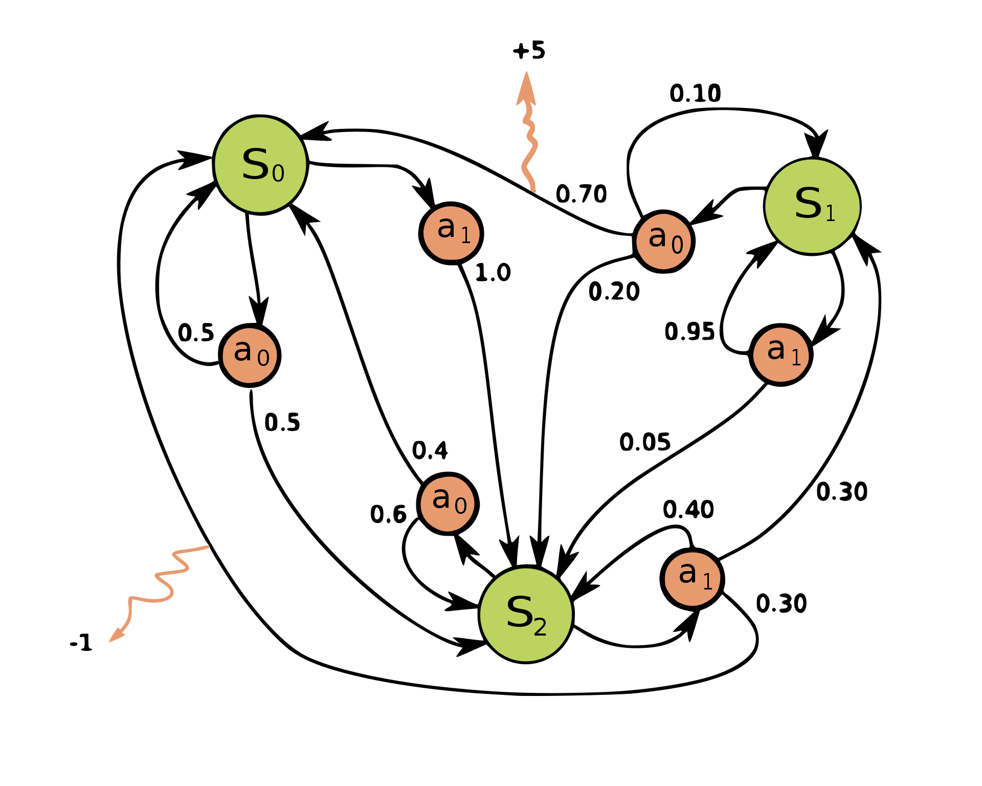
A simple MDP (credit to wikipedia). States can be seen in green and actions can be seen in red. Each state/action pair is associated with one or more transition probabilities to other states. The squiggly arrows show rewards emanating from certain state transitions being made.
To make this somewhat abstract definition of an MDP concrete, this is what a small portion of the transition function, $T$ would look like for the MDP defined in the diagram above:
| State | Action | Other State | Transition Probability |
|---|---|---|---|
| $S_0$ | $A_0$ | $S_0$ | 0.5 |
| … | … | … | … |
| $S_2$ | $A_1$ | $S_0$ | 0.3 |
You can imagine how the rest of the table would look. Similarly, a fragment of the reward function, $R$, would look as follows:
| State | Action | Other State | Reward Magnitude |
|---|---|---|---|
| $S_0$ | $A_0$ | $S_0$ | 0.0 |
| … | … | … | … |
| $S_2$ | $A_1$ | $S_0$ | -1.0 |
The definition of an MDP is intentionally very general. For example, the following situations could all be formalized as MDPs:
- A maze within a grid. Actions consist of N/E/S/W cardinal directions and states consist of valid grid positions. Rewards for transitioning to any position that is not the terminal maze position are small and negative. There is a large positive reward for reaching the terminal maze position.
- A game of chess. Actions are any valid action on a chess board, states are valid board positions. There is a positive reward for arriving at a winning game state and a negative reward for arriving at a losing game state.
- A self-driving car. Actions are to coast, accelerate, brake, turn left, turn right (and then combinations of those actions as well). The state consists of measurements of the car - current speed/acceleration, GPS position, heading, etc. There is a large positive reward for getting a passenger safely to their destination, a very large negative reward for crashing, hitting pedestrians, or breaking traffic laws.
We will talk about how MDPs are tied to reinforcement learning a bit later, but first will discuss two common algorithms for finding optimal state/action combinations within an MDP.
Values and policies? Some terminology
I make reference to the ideas of “values” and “policies” a lot in this post, but if you’re totally new to reinforcement learning, these terms aren’t necessarily helpful. A policy is how an agent chooses an action in a given state. The optimal policy is the best possible policy, where, for every state, we are choosing an action which maximizes the amount of reward we expect to obtain. Our goal is to find a policy that is as close to the optimal policy as possible. The policy is usually denoted as $\pi(s)$, and the optimal policy is denoted as $\pi_*(s)$.
The values of a state (or state-values) are the accumulated rewards that we expect to receive for being in state $s$ across the entire episode. The optimal value function tells us “if we were to act optimally according to our value estimates from this point onwards, this value represents the cumulative reward that we expect to receive.” Value functions are denoted as $V(s)$ and the optimal value function is denoted $V_*(s)$. You might worry about the optimal value for a state growing infinitely large if we find a policy containing a positive reward loop. For this reason, we use a “discounting” factor, $\gamma$, to denote “how much we value future reward”. On most tasks, we set $\gamma$ close to 1.0 (>0.9), so that we can look far ahead.
It is worth mentioning there are episodic (finite-time horizon) and non-episodic (infinite-time horizon) environments for MDPs, as well. Episodic environments contain a terminal state which requires us to restart from the beginning. An example of an episodic MDP would be chess, which ends when there is a win, loss, or draw. A non-episodic MDP would be traffic control, which has no end-of-episode trigger.
If you take one thing away from this blog post, it would be good to remember the Markov property. The Markov property states that an MDP is memoryless - this means that the best action given a state is completely independent of the states that came before it, and therefore, the best action depends only on the current state observations. This is desirable, since it removes (potentially expensive) conditioning on previous observations.
As an aside, although the reinforcement learning framework assumes the underlying mechanics of the task are an MDP, it has been shown empirically that some RL algorithms can still learn very good policies on tasks that do not satisfy the Markov property (such as arcade games - in pong, we do not know the trajectory of the ball from a single frame). Now that some basic terminology has been cleared up, let’s discuss the simple environment we intend to solve.
The Slippery Frozen Lake
The toy environment that will be used to demo MDP algorithms and reinforcement learning strategies is the slippery frozen lake environment. The environment works as follows:
- The environment is a square grid. Each grid cell represents a state in the MDP, which we will attempt to determine the value of.
- Every state has 4 actions (N, E, S, W). Walking into a wall is a valid action, but will just make you stay where you are.
- Because the lake is slippery, selected actions are only executed correctly 1/3 of the time. With 1/3 probability each, adjacent cardinal direction actions are taken. For example, if I choose to walk north, I will walk north with 1/3 probability, east with 1/3 probability, or west with 1/3 probability.
- There are no rewards except in terminal states. If we reach the goal, the reward is 1.0. If we fall in a hole, the reward is -1.0.
The optimal policy for this environment is one in which we eventually reach our goal, even if it takes us a very long time to do so. This means walking into walls a lot to avoid falling in the lake.
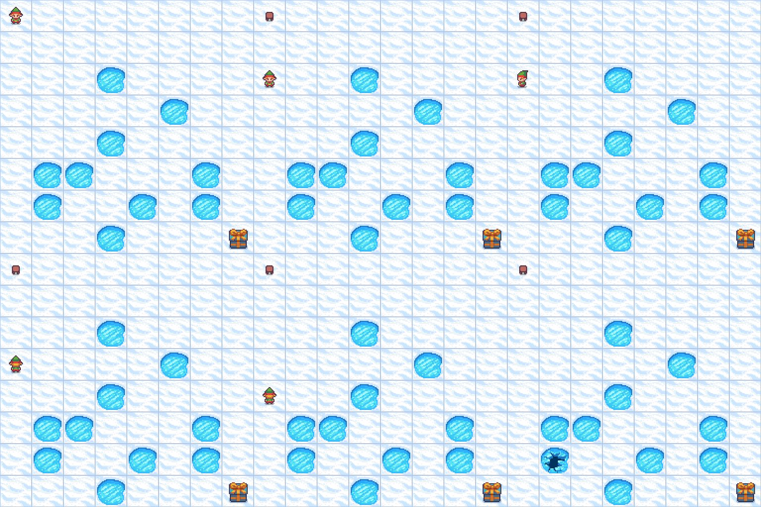
The untimely demise of our protagonist under a random policy.
So how do we find the safest route to our goal, given the uncertainty of our movement?
Exact Solutions to MDPs
This section introduces two algorithms that are used to solve MDPs exactly when their state- and reward-transition functions are known. This is almost never the case in practice, but these algorithms are interesting theoretically.
Value Iteration
The first approach to solving MDPs is an algorithm called value iteration. Value iteration initializes value estimates for each state randomly and then iteratively refines its value estimates using the following equation:
\[V(s) = \max_a \sum_{s'} T(s, a, s') * [R(s, a, s') + \gamma V(s')]\]What this means, effectively, is we iteratively use our previous estimate of $\textit{V}$ to eventually converge to the optimal value function, $V^{*}$. You may be wondering - how on earth does this work? We initialized $V$ as a bunch of random values, so how could this possibly converge to $V*$? The answer lies in the reward function - $R(s, a, s’)$. With each step of value iteration, the true rewards from the MDP are nudging our values closer to the true values of each state, making each state-value estimate monotonically better than the last.
When we iteratively apply this, within an infinite limit, the values will converge to the true values for each state. In practice, we can stop running value iteration if the largest difference between values from one step to the next is smaller than a manually chosen threshold (say, < 0.001 units, but this also problem-/reward-magnitude-dependent). We can also choose to stop value iteration if the optimal policy hasn’t changed in a fixed number of iterations.
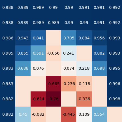
Optimal values found by value iteration for states in the frozen lake grid. Successful goal state with reward 1.0 is in the bottom right. All other states with no numbers are terminal non-goal states with -1.0 reward. Values for states that are guaranteed a reward of 1.0 are lower when they are further away from the goal state because of $\gamma$ discounting.
It’s worth mentioning that there is a one-to-one mapping from the optimal value function to the optimal policy. For each state, we choose the action that maximizes our expected future reward: \(a_{V*}=\mathop{\mathrm{argmax}}_a \sum_{s'} T(s, a, s') * [R(s, a, s') + \gamma V^*(s')]\).
Policy Iteration
Another algorithm for solving MDPs is called policy iteration. Policy iteration has similarities to value iteration, specifically in the policy evaluation step.
We begin by initializing a random policy. We then evaluate our policy in a way that is similar to value iteration (except instead of a max over actions, we assess the action that is chosen according to our current policy). This is the policy-evaluation step. The policy-evaluation step looks as follows:
\[V_{\pi_t}(s) = \sum_{s'} T(s, \pi_t(a), s') * [R(s, \pi_t(a), s') + \gamma V(s')]\]We run this iteratively in exactly the same way as value iteration until the largest magnitude difference between timesteps becomes smaller than a manually chosen threshold (note: this convergence criteria is exactly how value iteration converges). Once the policy-evaluation step has converged, we use our value estimates from the policy-evaluation step to improve the policy. This is the policy-improvement step:
\[\pi_{t+1}(s) = \mathop{\mathrm{argmax}}_a(\sum_{s'} T(s, a, s') * [R(s, a, s') + \gamma V(s')])\]Basically, the improved policy is the best action based on the value function that we just computed in the policy-evaluation step. The policy-improvement step is relatively quick compared to the policy evaluation step, since it only passes over each state once (as opposed to an arbitrary number of times). If the improved policy ends up being the same as the policy from the previous timestep, policy iteration has converged. If not, we use the improved policy as input to the policy evaluation step and repeat this evaluation $\rightarrow$ improvement step iteratively until the policy converges.
$$\pi_{0}(S) \rightarrow V_{\pi_0}(S) \rightarrow \pi_{1}(S) \rightarrow V_{\pi_1}(S) \rightarrow ... \rightarrow \pi_{*}(S)$$ Policy evaluation/improvement loop for policy evaluation.
The optimal policy that policy iteration (and also value iteration) converge to can be seen below:
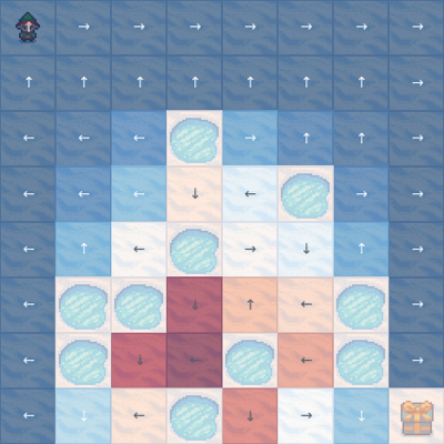
Optimal policy for policy/value iteration.
As you can see, the optimal policy rewards extreme caution. It is impossible to leave the perimeter of the map, but, without fail, in an infinite-time horizon, this policy will achieve the goal state and receive a reward of 1.0.
Reinforcement Learning
Policy iteration and value iteration both converge to the same optimal policy, since they are each guaranteed to find a solution to an MDP. While value/policy iteration are algorithms for solving MDPs when the transition and reward functions are fully accessible, practical problems are not usually formulated in this manner. In the real world, we usually operate through observations (sensor observations, etc.) and the underlying state-transition and reward mechanics are unknown to us. In the reinforcement learning problem, which more closely models the real world, we assume that we simply see a series of tuples $(s_t, a_t, r_{t+1}, s_{t+1})$ and we must act with no knowledge of $R$ or $T$. This means that we could the same action in the same state as before and get different results, without us fully understanding why. The process by which observation tuples are generated is shown below:
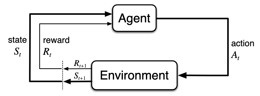
No blog post about RL is complete without this diagram. Diagram (and lots of other info) from Reinforcement Learning: An Introduction by Sutton & Barto.
How are MDPs and reinforcement related if we can’t see observe any internals of an MDP? Reinforcement learning assumes that an MDP is producing the observation tuples that we are seeing when we interact with the environment. Since we don’t have a $T$ or $R$ function available to us, we are faced with a more difficult problem and we need a new algorithm to account for our new uncertainty.
Enter: Q-Learning
Why is it called Q-learning? In Q-learning, we create a model of the quality of state-action pairs, which we call $Q(s, a)$. This is similar to a value function $V$, but now, we are considering a state-action value instead of just a state value. Q-Learning is even simpler than value iteration and policy iteration, but it takes much longer to converge. For a single observation tuple $(s_t, a_t, r_{t+1}, s_{t+1})$, this is the Q-learning update rule:
\[Q(s_t, a_t) = Q(s_t, a_t) + \alpha \cdot [(r_{t+1} + \gamma * \max_a{Q(s_{t+1}, a)}) - Q(s_t, a_t)]\]In this update rule, we choose $\alpha$, which is a “blending” parameter that governs how much we want our observation to influence our current estimate of $Q(s_t,a_t)$. Similarly as before, the $\gamma$ parameter governs how much we value future reward. This algorithm is similar to value iteration in that it iteratively refines its value estimates, but this time, we update them based on observations instead of a directly observed model of the MDP.
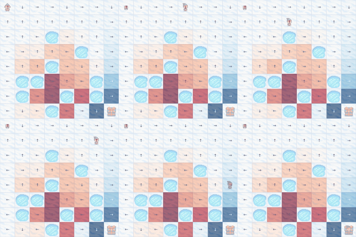
The er... meandering... Q-learning policy in action after 20k episodes. Note that some action choices are still not optimal - for example, first row, fifth column.
Although we create a “model” of the quality function, $Q$, Q-learning is confusingly not what is known as a “model-based approach”. Model-based approaches in reinforcement learning create a model of the state-transition- and reward-dynamics of the underlying MDP. Q-learning is model-free, because it does not create an explicit model of $T(s,a,s’)$ and $R(s,a,s’)$.
When training a Q-learning algorithm, the update rule is given above, but how do we choose actions to receive experience tuples to update our value estimates? If we always choose actions that we believe to be optimal, we will never know the value of states that our policy visits infrequently. However, if we only behave randomly, we may never actually execute an optimal policy and may be wasting time exploring when we already know how to act optimally. The trade-off between accumulating lots of reward and gaining information about not-yet-visited states is called the exploration-exploitation dilemma. We should choose actions so that we can balance exploration with optimizing reward.
A simple and widely used algorithm for choosing actions for Q-learning is called $\epsilon$-greedy action selection. $\epsilon$-greedy action selection states that we should choose an action randomly with probability $\epsilon$ or otherwise, with probability $1-\epsilon$, we choose an action from the policy given by our current estimation of $Q(s, a)$. It is common practice to reduce $\epsilon$ ($\epsilon$-decay) over time to decrease the rate of random action selection as our policy improves.
Value iteration converges in 643 steps, policy iteration in 10 steps, and Q-learning in 20000 episodes (and not even to the optimal policy for every grid square). These aren’t extremely meaningful comparisons since the steps of each algorithm take a variable amount of computation time, but it’s clear that twenty-thousand episodes for practical RL applications would require a lot of time in the real world. Even if time isn’t an issue, most real-world control problems wouldn’t have the tolerance for twenty-thousand episodes worth of mistakes.
Beyond Q-Learning
Of course, the slippery frozen lake is incredibly simple compared to many real-world reinforcement learning problems. Many real-world applications use continuous-valued sensor measurements as state measurements. Because continuous-valued sensor measurements are much more varied and represent a massive number of states when combined, it becomes intractable to create a Q value for every state-action pair. In this case, we prefer to approximate Q-values with a flexible function approximator, such as a neural network. This approach is called Deep Q-Learning. There are some tricks that are needed to get Deep Q-Learning working, but it is an incredible algorithm that has been used to play video games at superhuman levels from just pixel data1. If you’re interested in going deeper learning about reinforcement learning, the most comprehensive guide, as of writing this, is Reinforcement Learning: An Introduction by Sutton & Barto. Thanks for reading!