Re-writing Micrograd: Training a Neural Network from Scratch
The code associated with this blog post can be found here.
Table of Contents
- Background
- Neural Networks
- Computational graphs
- Calculus
- Gradients on a Computational Graph
- The Other Parts of Training a Neural Network
- Training a Network!
- Conclusion
Background
In an attempt to refamiliarize myself with the backpropagation algorithm (i.e. “backprop”), I re-wrote an autograd library written by Andrej Karpathy called “micrograd”, and (almost successfully) managed to do so without looking. Micrograd runs reverse-mode automatic-differentiation (auto-diff) to compute gradients for a computational graph. Since a neural network is a special case of a computational graph, backprop is a special case of reverse-mode auto-diff when it is applied to a neural network. If this sounds confusing, read on, and I will break this all down step-by step.
You will need a bit of calculus knowledge of elementary derivatives and the chain rule to understand this. If you have previously studied calculus but need a refresher, this post should get you up to speed on what you need to remember. There’s, unfortunately, no way to make a post about backpropagation short, but I have provided a table of contents so you can skim/skip sections that you’re already familiar with.
This is an informal post that will use some formal math notation, mostly derivatives. I almost always prefer code and visuals to math notation, but sometimes it can’t be helped.
If you somehow arrived here without having seen Andrej Karpathy’s original video, I highly recommend you check out the original here.
Neural Networks
If you aren’t familiar with why neural networks are a big deal, I could write thousands of words on that, but I will spare you. Neural networks are non-linear (e.g. any function that’s not a line, think \(y=x^2\)) function approximators that can theoretically approximate any continuous function. They can be used to model statistical co-occurrences of words (as in large language models), used to model co-occurrences of image pixels (as in image segmentation/classification models), used to help recommend content on a website (via content embeddings), and are an important component of systems that can play games at superhuman levels (as in deep reinforcement learning). Each of these things are extremely cool in their own right and deserve a blog post of their own, but this post is going low-level in how simple neural networks are trained via backpropagation and gradient descent.
Maybe not... superhuman performance... but a moderately smart reinforcement learning agent I trained using a deep Q-network with experience replay.
The most amazing thing about neural networks to me is that however different the network purposes are, they are all trained with one common algorithm - that algorithm is backpropagation. GPT-4 is trained using backpropagation. All sorts of generative AI (e.g. stable diffusion, midjourney) are trained with backpropagation. Even local image explanations in the emerging field of explainable AI are produced using backpropagation (on the input pixels of the image instead of the network weights). It’s not an exaggeration to say that recently, backpropagation has become one of the most important algorithms in the world.
In brief: neural networks are function approximators that take an input X and produce a predicted output Y that attempts to model a true distribution of the input data. There is a training procedure called backpropagation that, when combined with gradient-based optimization algorithms, iteratively drives the neural network’s approximation closer to the true function it is trying to approximate. The data the network is fed, the architecture, and the loss function of a neural network primarily govern how it behaves. If any of this is confusing to you, there is a beautiful introduction to neural networks by 3blue1brown. Otherwise, lets discuss computational graphs.
Computational graphs
What is a computational graph?
A computational graph is a directed acyclic graph (DAG) in which nodes correspond to either variables or operations. The simplest computational graph might look as follows:

A computational graph in its simplest form - two variables: a=1 and b=2 being multiplied to produce a third value, c=2. The code to generate these visuals was adapted from Andrej's graphviz code in Micrograd.
While this is a very simple example of a computational graph, it’s a step in the right direction for what we need for a forward pass in a neural network. It might help to show what a single neuron activation looks like in a computational graph and compare it to the more “classic” representation of a neural network.
Representing (Simple) Neural Networks as a Computational Graph
You have probably seen a traditional view of a neural network as a bunch of tangled edges between nodes in an undirected graph. While this is a compact way to represent neural networks visually, for the purposes of backpropagation, it’s much better to think of the network as a computational graph.
Let’s pretend that we have a very, very small neural network with two inputs, two hidden nodes, and a single output. Let’s also pretend that we have just computed the activation for a single neuron in the hidden layer, h1. In the graph, we will assume dark gray nodes have triggered as of the present time and light gray nodes have not yet triggered. Here’s what the traditional view of this might look like:

A neural network in which we have just computed $$h_1=tanh(x_1w_1+x_2w_2)$$
The equivalent computational graph, representing just \(h1\)’s activation, would look as follows:
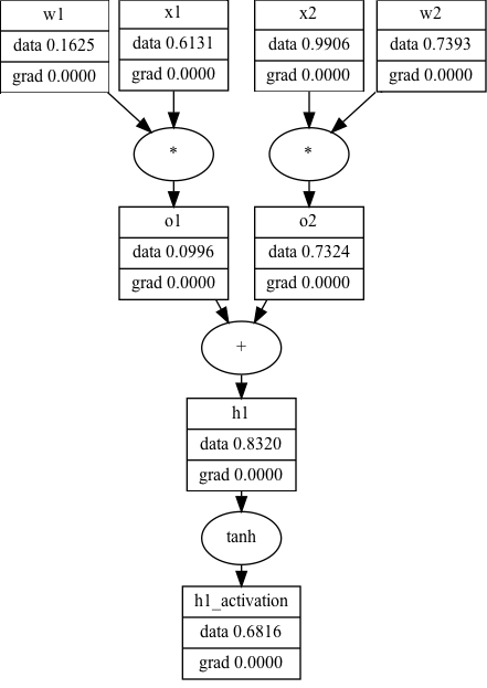
While the computational graph view is a lot less… terse… it makes explicit a number of details that the traditional view of neural networks obscure. For example, you can see, step-by-step, the process of computing a neuron’s activation:
- Multiply the inputs by the neuron’s weights (\(o_1=w_1x_1; o_2=w_2x_2\))
- Sum all of the \(wx\) terms (\(h_1=o_1+o_2\))
- Compute the activation for \(h1\) (\(h_1\_activation=tanh(h1))\)
It’s unclear that all of this is happening in the first view. More importantly, the computational graph allows us to show what the data (and the gradients, but more on that later) are at each step of the way. You can imagine that if this is one neuron (h1), all the other neurons in a hidden layer (in this case, h2) fire the same way with different weights. Now that you have seen how computational graphs can be used to represent neural networks, we’re going to put this on hold for a second and take a trip back to Calc 1.
Calculus
Because we want to find out how we can change the weights of a neural network to make its performance improve, we will need to calculate the gradient of the weights with respect to some sort of performance measurement (known as the loss, but more on that later). You will need to know a few elementary derivatives and have an intuitive grasp of the chain rule to understand how backpropagation works. Both of those things will be covered in brief here.
Derivatives for a Simple Feedforward Network
For this tutorial, we are considering a feedforward neural network with one input layer (i.e. data), a hidden layer, and an output layer. The derivatives that you need to know for this network are: addition, multiplication, tanh, and the power function. The derivatives for these are as follows:
Addition: \(f(x, y)=x+y\); \(\frac{\partial f}{\partial x}=1; \frac{\partial f}{\partial y}=1\)
Multiplication: \(f(x, y)=xy\); \(\frac{\partial f}{\partial x}=y; \frac{\partial f}{\partial y}=x\)
Tanh: \(f(x)=\frac{e^x-e^{-x}}{e^x+e^{-x}}\); \(\frac{d f}{d x}=1-\tanh(x)^2\)
Pow: \(f(x, y)=x^y\); \(\frac{\partial f}{\partial x}=y * x^{(y-1)}\)
(leaving out the derivative \(\frac{\partial f}{\partial y}\) for the power function, because I’m being lazy and it’s not important for the purposes of this post)
Chain rule
The amount of times that I’ve heard backpropagation described as a “recursive application of the chain rule” without the explainer providing intuition about what that actually means makes my head spin. In the Andrej’s video where he covers backpropagation, he references Wikipedia’s explanation of the chain rule, which I think is one of the most cogent explanations of a topic that is frequently over-complicated in the context of backpropagation. Specifically, Wikipedia says:
If a variable z depends on the variable y, which itself depends on the variable x (…), then z depends on x as well, via the intermediate variable y. In this case, the chain rule is expressed as \(\frac{d z}{d x}=\frac{d z}{d y}\frac{d y}{d x}\)
Effectively, we are able to simply multiply the rates of change if we have \(\frac{d z}{d y}\) and \(\frac{d y}{d x}\) to get \(\frac{d z}{d x}\). Although \(\frac{d z}{d y}\) isn’t really a fraction, an easy way to remember this is that \(d y\) terms still “cancel each other out” as though they were fractions.
The Wikipedia page offers a concrete example, as well. Specifically, it asks us to consider the speed of a human, a bicycle, and a car. Lets say \(h\) represents the speed of a human, \(b=2h\) the speed of the bicycle, and \(c=4b\) the speed of the car. We want to find the rate of change of the car with respect to the human. We can calculate \(\frac{d c}{d b} = 4\) and \(\frac{d b}{d h} = 2\) and by the chain rule, we know that \(\frac{d c}{d h} = \frac{d c}{d b} \frac{d b}{d h} = 4 * 2 = 8\), or that a car is 8 times as fast as a human.
In the context of backpropagation, for an arbitrary weight, we have a gradient that flows into the current network weight from somewhere further down the computational graph (i.e. it is “backpropagated”). This value represents how all of the downstream activations that the current weight feeds into affect the loss. Since the performance of the network is affected by all the activations downstream that the current weight affects, we need to look how it indirectly affects the loss through the nodes that it contributes to downstream. The chain rule gives us a way to compute this value. We must multiply the “global” derivative that has been propagated backwards with the “local” derivative of the current weight. Once we do this, the current node’s derivative becomes the new “global” derivative and we continue to pass the new “global” derivative backwards. This is what is meant by “recursively applying the chain rule”. You don’t have to understand all of this now, and it should become clear with a spelled out example in the next section.
Gradients on a Computational Graph
Now that we’ve covered the relevant bits of calculus and computational graphs, we are going to combine them to take derivatives on a computational graph using the chain rule. We will first go over a graph that is one node deep and then we will make it deeper so that we are forced to use the chain rule to propagate gradients using the chain rule.
The Trivial Case
Let’s look at the simplest form of a computational graph that we made above. We want to compute the derivative of \(c\) with respect to \(a\) and \(b\). We know trivially that as \(c\) changes, \(c\) varies proportionally to it. The derivative of any function with respect to itself is 1: \(\frac{dc}{dc} = 1\). We can fill this out in our computational graph:

We know that \(c(a, b) = a \cdot b\) and, further that \(\frac{\partial c}{\partial a} = b\). By the same logic, \(\frac{\partial c}{\partial b} = a\). In a computational graph, when backpropagating gradients, the multiplication operator acts as a magnitude/gradient “swap” that magnifies the current input’s gradient by the other input’s magnitude. This makes sense - if the current value is a result of a multiplication operation and it grows, the output value grows proportionally to the value that it’s multiplied by. The final graph looks like this:

Note that b took a’s data as its gradient and vice versa. The full operations that are happening here are \(\frac{d c}{d c}\frac{\partial c}{\partial a} = 1.0 * b = 2.0\) and \(\frac{d c}{d c}\frac{\partial c}{\partial b} = 1.0 * a = 1.0\), since we are multiplying the “local” gradients of \(a\) and \(b\) by the downstream gradient, \(\frac{dc}{dc} = 1\). The code to implement the multiplication operation for a computational graph in python is this simple:
def mul(self, other):
    """Multiplies two values together and configure result to compute gradient"""
    if isinstance(other, (int, float)):
        other = Value(other)

    def backward():
        """
        Multiply "swaps" magnitudes from inputs and multiplies upstream grad
        """
        self.grad += other.data * result.grad
        other.grad += self.data * result.grad

    result = Value(data=self.data * other.data, children=(self,other), _backward=backward)
    return result
Without going too much into the definition of the Value class (it’s a data node in a computational graph), a new value is created (in our case, c). When c._backward() is called, it does exactly what we just described - the inputs to the multiplication operation (self and other) take the other input’s data as a gradient, multiplied by the downstream gradient (result.grad - in this case, 1.0). The reason we use the += operator is because we are accumulating gradients rather than resetting them - a node in the computational graph often feeds into many downstream nodes.
The next computational graph example should help make the gradient flow more concrete.
Two Levels Deep - Propagating Gradients
Since we are working with neural networks, let’s look at a common operation: multiplying weights and inputs (\(w_i\) and \(x_i\)) and then taking their sum (we will skip the activation function for now). Similar to the hidden unit that we expressed above, let’s look at two inputs and two weights feeding into a hidden node, \(h1\). We already know that, trivially, \(\frac{d_{h1}}{d_{h1}} = 1\), but to make the gradient flow clearer, let’s pretend that h1 is nested in a larger graph and that it received a gradient value of 2.0 with respect to some downstream variable that we aren’t concerned with.

In calculating \(\frac{d_{h1}}{d_{o1}}\) and \(\frac{d_{h1}}{d_{o2}}\), we need to look to the addition derivative function: \(f(o1, o2)=o1+o2\); \(\frac{d_{h1}}{d_{o1}}=1.0\); \(\frac{d_{h1}}{d_{o1}}=1.0\). Each input to the addition operation has a local gradient of 1. This means any downstream gradient is multiplied with magnitude 1.0 into the current node - the addition operation just passes on the gradient unchanged and effectively acts as a gradient “splitter”. The code to implement addition is similarly simple to multiplication:
def add(self, other):
    """Add two values together and assign local gradient"""
    if isinstance(other, (int, float)):
        other = Value(other)

    def backward():
        """
        Add "splits" gradients from result back to current node.
        """
        self.grad += 1.0 * result.grad
        other.grad += 1.0 * result.grad

    result = Value(self.data + other.data, children=(self,other), _backward=backward, _op='+')
    return result
For each input to the addition function (self and other), we assign the gradient for the local nodes as the gradient that we receive from result times 1.0 - this gives us our “splitter” behavior. Adding behavior in the computational graph is very easy to remember.
When we multiply the downstream gradient at \(h1\) (2.0) into the current node (o1 or o2) with magnitude 1.0 (because of the addition operation), we get (1.0 * 2.0) = 2.0. This is the chain rule! We multiplied the magnitude of the downstream “global” gradient by the current node’s “local” gradient. After following these steps, the computational graph now looks as follows:

Continuing backpropagation into the next layer, next we have multiplication operations, which we are already familiar with. To get the gradients for our inputs, we can apply the chain rule to the intermediate gradients that we’ve just computed, and then we simply multiply. Let’s look at the gradient for \(\frac{d_{h1}}{d_{w1}}\). If we have \(\frac{d_{h1}}{d_{o1}}\) and \(\frac{d_{o1}}{d_{w1}}\), we have everything we need: \(\frac{d_{h1}}{d_{w1}}=\frac{\partial_{h1}}{d_{o1}}\frac{d_{o1}}{d_{w1}}\). We just need to calculate the local derivative, \(\frac{d_{o1}}{d_{w1}}\). We know that \(o1 = w1 \cdot x1\), and therefore, that \(\frac{d o1}{d w1} = x1\). So we get \(\frac{d_{h1}}{d_{w1}}=\frac{d_{h1}}{d_{o1}}\frac{d_{o1}}{d_{w1}}= \frac{d_{h1}}{d_{o1}} \cdot x1.data = 2.0 \cdot 2.0 =4.0\). This means that when we increase \(w1\) by 1.0, the node that we are calculating the gradient with respect to (the one that we aren’t concerned with, somewhere downstream beyond h1) increases by 4.0 units. We can apply the same logic to the other inputs to calculate all of the gradients:

There is a lot of derivative notation here, but it really just says that you multiply the “local gradient” by the gradient that flows back to it from further down the graph.
Here’s the magic of it: as long as you can calculate the derivative of a function, you can include it in the computational graph and compute the gradient for inputs to that function. Every common neural network operation is differentiable for this reason! A simple neural network forward pass might consist of multiplication –> addition –> (differentiable) non-linearity –> multiplication –> addition –> loss function.
The reason this is called reverse-mode autodiff is because we have to compute a forward pass to cache the “data” values, and then, we start from the end and use the cached forward data values in our derivative calculations while we work backwards. There is also a form of autodiff called forward-mode autodiff, but it makes more sense when there are more outputs than inputs, which is usually not the case with neural networks.
This is all you need to understand backpropagation. While I’m glossing over the many network weights that feed into an activation in a hidden layer and the activation function, you can imagine it’s more of the same as what we’ve already done with different derivatives1. With the gradients of the weights, we’re ready to do something powerful. What if we could tweak the weights so that the output goes up or down? This is where gradient descent comes in.
The Other Parts of Training a Neural Network
In addition to taking derivatives on a computational graph, we need something that helps us determine how good our predictions are and a way to tweak our network so that the predictions get closer to “good”. This section discusses those two aspects of training a neural network.
Loss Functions
The ultimate goal of a neural network is to make accurate predictions. In order to assess how well the network makes predictions, we need to consider a loss function, which, given a prediction and a true label, scores how close the network was to being correct. If the network is performing poorly, the loss will be high, and if the network is performing well, the loss will be low. Usually, the final output of the network will be this loss function, and the loss function is almost always differentiable. If you are doing regression or classification, you will always have a loss function as the final node in your neural network’s computational graph.
As an example, let’s look at mean-squared error (MSE) - a common loss function used in linear regression:
\[MSE=\frac{1}{n} \sum_{i=1}^n{(Y_i - \hat{Y_i})^2}\]\(n\) is the amount of input training examples, \(Y_i\) is the true label and \(\hat{Y_i}\) is the predicted label outputted by our network. Let’s examine a few simple cases where \(n=1\). When we predict a label of 1.0, but the true label is 0.0, we get a loss of 1.0. Similarly for when we predict a label of 0.0 and the true label is 1.0. As the prediction gets closer to the loss, the average mean-squared error of outputs gets smaller, driving our predictions closer to the true label. Since a neural network ending with MSE is composed entirely of differentiable functions, we can calculate the derivatives of weights at any depth with respect to the loss function in order to change the weights to drive the loss downward. When we calculate gradients with respect to the loss, we are figuring out how we can make our predictions (\(\hat{Y_i}\)) closer to the true function (\(Y_i\))!
Note that to compute MSE, we only need to compute the derivatives for \(f(x)=x ^ 2\) and \(f(x, y) = x - y\). We could calculate a derivative for MSE and make it its own function, or we could make the computational graph a bit deeper and perform those operations separately. In an autograd engine, it doesn’t matter the level of granularity that you calculate derivatives for - as long as the function is differentiable, we can calculate \(f(x, y) = (x - y) ^ 2\) or separately calculate \(z=x-y\) and then feed it into \(f(z)=z^2\) afterwards.
Gradient Descent
Once we have calculated the loss, we backpropagate from the end of the graph to calculate gradients for all nodes in the graph. Since the gradients are in the direction of the positive loss, we need to tweak the values of the weights in the opposite direction of the gradient, since we are trying to drive the loss towards 0. The naive gradient descent algorithm is extremely simple: once we have the gradients for the weights, move each weight in the opposite direction of the gradient a very small amount (i.e. 0.01). The small amount that we move it is called the learning rate, and is an important parameter for tuning neural networks. In our previous example, the output of a step of gradient descent for the single training example (consisting of (x1, x2)) would look as follows:

In this case, we used the learning rate \(\alpha=0.01\). W2 was twice as affected than W1 by the gradient descent step because it has 2x larger gradient. We have also completed a new forward pass and can observe the new output of \(h1\) is lower than it previously was! If \(h1\) were a loss function, we would have made the network’s predictions closer to the true function we are trying to model.
This is a simplified example, but it’s really not that much different from what your neural network libraries like PyTorch and Tensorflow are doing in practice. They’re just much better at parallelizing gradient computations and batching your data to do fancier things like mini-batch gradient descent. There is a fair amount we didn’t cover with neural network training here (such as different types of loss functions, different gradient-based optimization algorithms, actually implementing a full neural network), but that isn’t important for understanding how a neural network is trained at a low level. Now, I’ll show you some neural networks I trained from scratch using my autodiff library.
Training a Network!
I debated whether or not to include this, since it’s not immediately related to backpropagation, but I figured it would be cool to show the reward for implementing an autodiff engine. This is an evolving decision boundary of a neural network that was hand-coded with no external dependencies in python. It’s orders of magnitude slower than pytorch would be for the same thing, but it does (more or less) exactly the same thing without the massive parallelization and numerical stability precautions.
The function that I am trying to model is whether or not a point is within a circle with radius 1.0 centered on (0,0). I generated approximately equal parts positive and negative training data. The non-linearity that I used was tanh and the loss function was mean-squared error. Here are networks trained with 1, 2, and 9 hidden neurons - the points plotted from each class are from the training set:

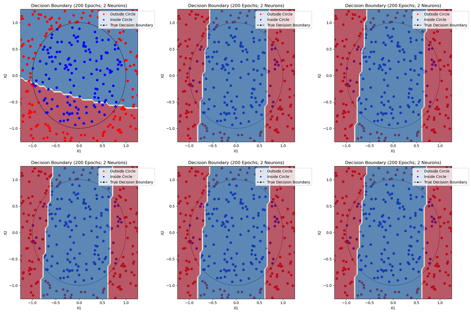

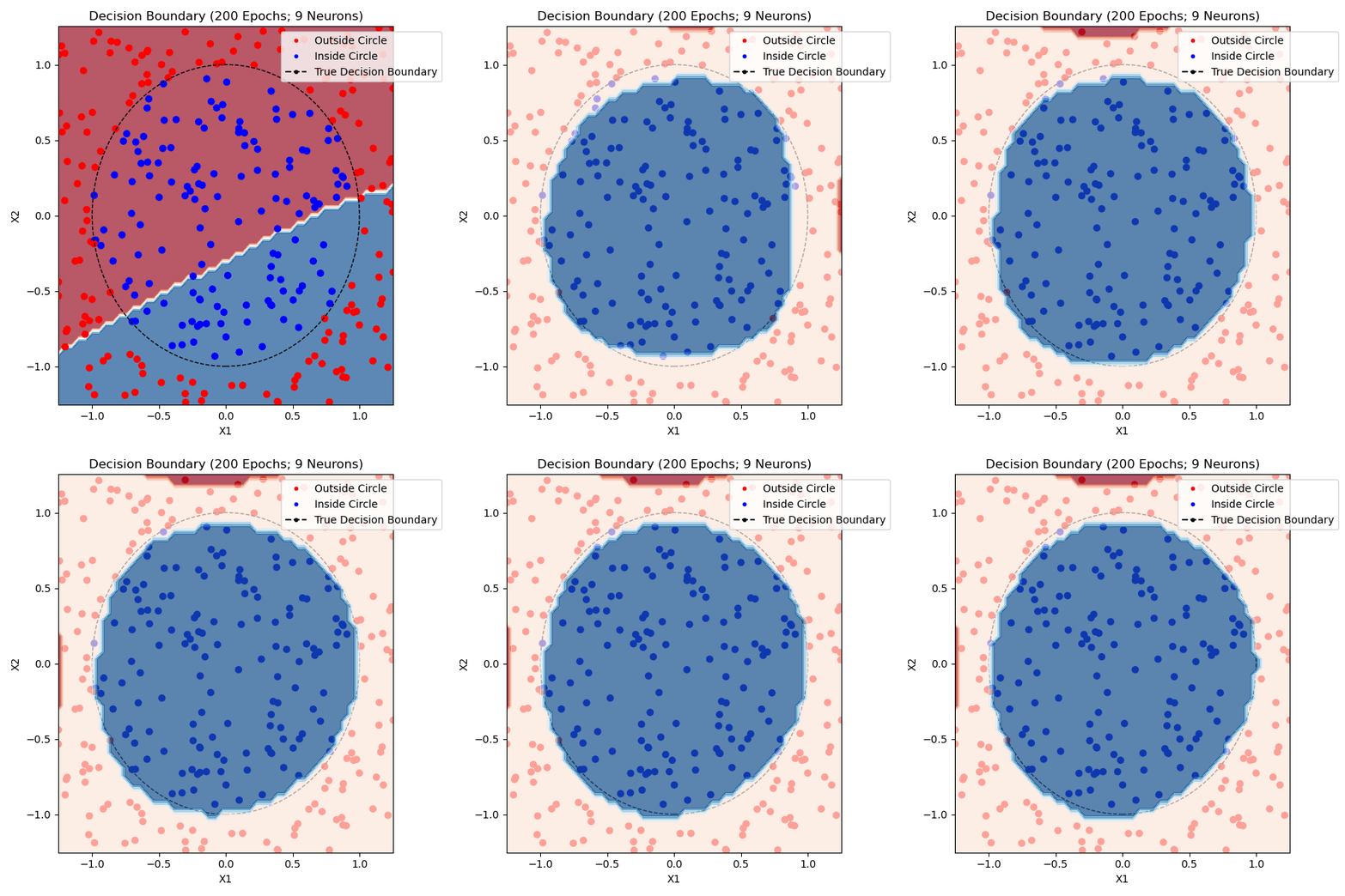
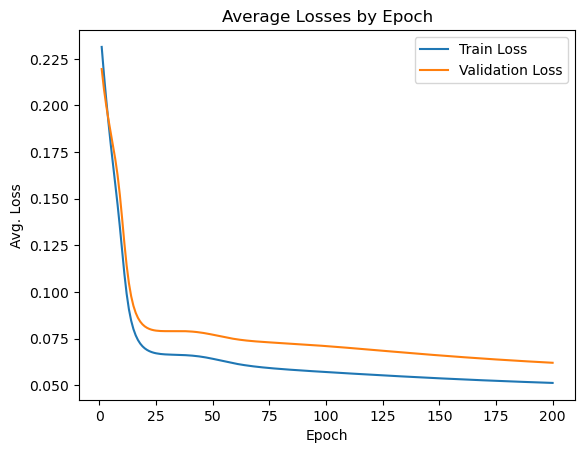
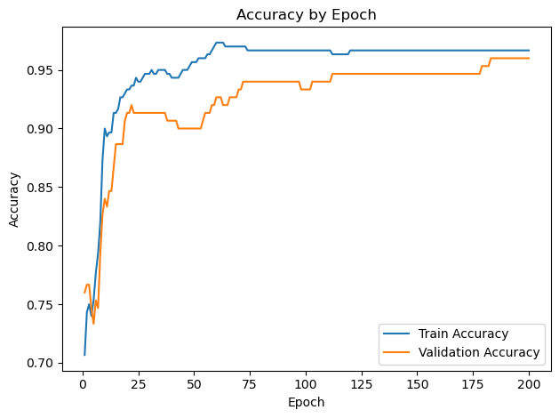
You can see that one neuron can only roughly approximate a linear decision boundary, two extends that to a parabola, three actually has enough representative power to model a crude circle, and nine has the representative power to model a fairly precise circle. And this was all done with python built-in libraries! Of course, no blog post about training a neural network would be complete without the loss and accuracy per epoch for the (9-hidden neuron) network, which is standard practice to plot to see if there is a bottleneck in network training:
Conclusion
It’s easier to consider a computational graph separate from a neural network than it is to go through each individual weight in a neural network in excruciating detail when explaining backpropagation. Once you see how the “local derivatives” and the “global derivatives” work together and how the chain rule is recursively applied on a small scale, it’s not a big step to go from our example to a full feedforward network. This was long, but I hope it gave a good framework to approach and debug neural network training. Thanks for reading!
If you have anything to add or see anything that you believe may be incorrect, please contact me at will@willbeckman.com.