Backpropagation

The code associated with this blog post can be found here.

Table of Contents

Background

In an attempt to refamiliarize myself with the backpropagation algorithm (i.e. “backprop”), I re-wrote an autograd library written by Andrej Karpathy called “micrograd”, and (almost successfully) managed to do so without looking. Micrograd runs reverse-mode automatic-differentiation (auto-diff) to compute gradients for a computational graph. Since a neural network is a special case of a computational graph, backprop is a special case of reverse-mode auto-diff when it is applied to a neural network. If this sounds confusing, read on, and I will break this all down step-by step.

You will need a bit of calculus knowledge of elementary derivatives and the chain rule to understand this. If you have previously studied calculus but need a refresher, this post should get you up to speed on what you need to remember. There’s, unfortunately, no way to make a post about backpropagation short, but I have provided a table of contents so you can skim/skip sections that you’re already familiar with.

This is an informal post that will use small amounts of formal math notation, but I will try in keep it to a minimum. In places where math notation could be used, I prefer visuals and code.

If you somehow showed up here without having seen Karpathy’s original video, I highly recommend you check out the original here.

Neural Networks

If you aren’t familiar with why neural networks are a big deal, I could write thousands of words on that, but I will spare you. Neural networks are non-linear function approximators that can theoretically approximate any continuous function. They can be used to model statistical co-occurrences of words (as in large language models), they can be used to model co-occurrences of image pixels (as in image segmentation/detection/classification models), they can be used to help recommend content on a website (via content embeddings), and they are an important component of systems that can play games at superhuman levels (as in deep reinforcement learning). Each of these things are extremely cool in their own right and deserve a blog post of their own, but this post is going low-level in how neural networks are trained.

Maybe not... superhuman performance... but a moderately smart reinforcement learning agent I trained for class using a deep Q-network with experience replay.

The most amazing thing about neural networks to me, however, is that they are all trained with a single algorithm. As you might have guessed, that algorithm is backpropagation. GPT-4 is trained using backpropagation. All sorts of generative AI (e.g. stable diffusion, midjourney) are trained with backpropagation. Even local image explanations in the emerging field of explainable AI are produced using backpropagation (on the input pixels of the image instead of the network weights). It’s not an exaggeration to say that recently, backpropagation has become one of the most important algorithms in the world.

So in brief: neural networks are function approximators that take an input X and produce a predicted output Y that attempts to model a true distribution of the input data. There is a training procedure called backpropagation that iteratively drives the neural network’s approximation closer to the true function it is trying to approximate. The data the network is fed, the architecture, and the loss function of a neural network primarily govern how it behaves. If any of this is confusing to you, you might want to brush up on how neural networks work with a supplemental resource like 3blue1brown. Otherwise, lets discuss computational graphs.

Computational graphs

What is a computational graph?

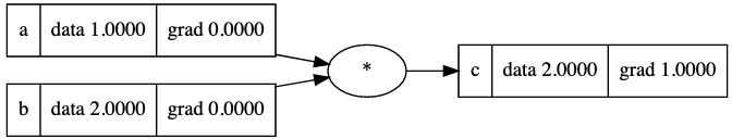
A computational graph is a directed acyclic graph (DAG) in which nodes correspond to either variables or operations. The simplest computational graph might look as follows:

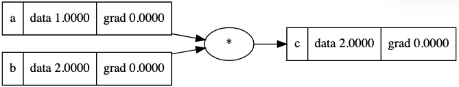
A computational graph in its simplest form - two variables - a=1 and b=2 being multipled to produce a third value, c=2. The code to generate these visuals was adapted from Karpathy's code in Micrograd.

While this is a very simple example of a computational graph, it’s a step in the right direction for what we need for a forward pass in a neural network. It might help to show what a single neuron activation looks like in a computational graph and compare it to the more “classic” representation of a neural network.

Representing (Simple) Neural Networks as a Computational Graph

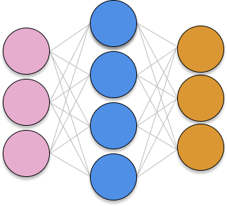
You have probably seen a traditional view of a neural network as a bunch of tangled lines between nodes. While this is a compact way to represent neural networks visually, for the purposes of backpropagation, it’s much better to think of the network as a computational graph.

Let’s pretend that we have a very, very small neural network with two inputs, two hidden nodes, and a single output. Let’s also pretend that we have just computed the activation for a single neuron in the hidden layer, h1. In the graph, we will assume dark gray nodes have triggered as of the present time and light gray nodes have not yet triggered. Here’s what the traditional view of this might look like:

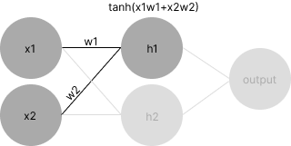
A neural network in which we have just computed

h_{1} = t a n h (x_{1} w_{1} + x_{2} w_{2})

$h_1=tanh(x_1w_1+x_2w_2)$

The equivalent computational graph, representing just $h1$ ’s activation, would look as follows:

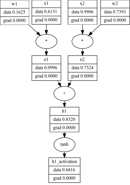
While the computational graph view is a lot less… terse… it makes explicit a number of details that the traditional view of neural networks obscure. For example, you can see, step-by-step, the process of computing a neuron’s activation:

Multiply the inputs by the neuron’s weights ( $o_1=w_1x_1; o_2=w_2x_2$ )
Sum all of the $wx$ terms ( $h_1=o_1+o_2$ )
Compute the activation for $h1$ ( $h_1\_activation=tanh(h1))$

It’s unclear that all of this is happening in the first view. More importantly, the computational graph allows us to show what the data (and the gradients, but more on that later) are at each step of the way. You can imagine that if this is one neuron (h1), all the other neurons in a hidden layer (in this case, h2) fire the same way with different weights. Now that you have seen how computational graphs can represent neural networks, we’re going to put this on hold for a second and take a trip back to Calc 1.

Calculus

Because we want to find out how we can change the weights of a neural network to make its performance improve, we will need to calculate the gradient of the weights with respect to some sort of performance measurement (known as the loss). You will need to know a few elementary derivatives and have an intuitive grasp of the chain rule to understand how backpropagation works. Both of those things will be covered in brief here.

Derivatives for a Simple Feedforward Network

For this tutorial, we are considering a feedforward neural network with one input layer (i.e. data), a hidden layer, and an output layer. The derivatives that you need to know for this network are: addition, multiplication, tanh, and the power function. The derivatives for these are as follows:

Addition

f (x, y) = x + y

$f(x, y)=x+y$

\frac{\partial f}{\partial x} = 1; \frac{\partial f}{\partial y} = 1

$\frac{\partial f}{\partial x}=1; \frac{\partial f}{\partial y}=1$

Multiplication:

f (x, y) = x y

$f(x, y)=xy$

\frac{\partial f}{\partial x} = y; \frac{\partial f}{\partial y} = x

$\frac{\partial f}{\partial x}=y; \frac{\partial f}{\partial y}=x$

Tanh:

f (x) = \frac{e^{x} - e^{- x}}{e^{x} + e^{- x}}

$f(x)=\frac{e^x-e^{-x}}{e^x+e^{-x}}$

\frac{d f}{d x} = 1 - \tanh (x)^{2}

$\frac{d f}{d x}=1-\tanh(x)^2$

Pow:

f (x, y) = x^{y}

$f(x, y)=x^y$

\frac{\partial f}{\partial x} = y * x^{(y - 1)}

$\frac{\partial f}{\partial x}=y * x^{(y-1)}$

(leaving out the derivative $\frac{\partial f}{\partial y}$ for the power function, because I’m being lazy and it’s not important for our purposes)

Chain rule

The amount of times that I’ve heard backpropagation described as a “recursive application of the chain rule” without the explainer providing intuition about what that actually means makes my head spin. In the Andrej’s video where he covers backpropagation, he references Wikipedia’s explanation of the chain rule, which I think is one of the most cogent explanations of a topic that is frequently over-complicated in the context of backpropagation. Specifically, Wikipedia says:

If a variable z depends on the variable y, which itself depends on the variable x (…), then z depends on x as well, via the intermediate variable y. In this case, the chain rule is expressed as $\frac{d z}{d x}=\frac{d z}{d y}\frac{d y}{d x}$

Effectively, we are able to simply multiply the rates of change if we have $\frac{d z}{d y}$ and $\frac{d y}{d x}$ to get $\frac{d z}{d x}$ . Although $\frac{d z}{d y}$ isn’t really a fraction, the $d y$ terms “cancel each other out” in the same way in this context.

The Wikipedia page offers a concrete example, as well. Specifically, it asks us to consider the speed of a human, a bicycle, and a car. Lets say $h$ represents the speed of a human, $b=2h$ the speed of the bicycle, and $c=4b$ the speed of the car. We want to find the rate of change of the car with respect to the human. We can calculate $\frac{d c}{d b} = 4$ and $\frac{d b}{d h} = 2$ and by the chain rule, we know that $\frac{d c}{d h} = \frac{d c}{d b} \frac{d b}{d h} = 4 * 2 = 8$ , or that a car is 8 times as fast as a human.

In the context of backpropagation, for an arbitrary weight, we have a gradient that flows into the current weight from somewhere further down the graph. This value represents how all of the downstream activations that the current weight feeds into affect the loss. Since the performance of the network is affected by all the activations downstream that the current weight affects, we need to look how it indirectly affects the loss through the nodes that it contributes to downstream. The chain rule gives us a way to compute this value. We must multiply the “global” derivative that has been propagated backwards with the “local” derivative of the current weight. Once we do this, the current node’s derivative becomes the new “global” derivative and we continue to pass the new “global” derivative backwards. This is what is meant by “recursively applying the chain rule”. You don’t have to understand all of this now, and it should become clear with a spelled out example in the next section.

Gradients on a Computational Graph

Now that we’ve covered the relevant bits of calculus and computational graphs, we are going to combine them to take derivatives on a computational graph using the chain rule. We will first go over a graph that is one node deep and then we will make it deeper so that we are forced to use the chain rule to propagate gradients using the chain rule.

The Trivial Case

Let’s look at the simplest form of a computational graph that we made above. We want to compute the derivative of $c$ with respect to $a$ and $b$ . We know trivially that as $c$ varies, $c$ varies proportionally to it. The derivative of any function with respect to itself is 1:

\frac{d c}{d c} = 1

$\frac{dc}{dc} = 1$

We can fill this out in our computational graph

We know that $c(a, b) = a \cdot b$ and, further that $\frac{\partial c}{\partial a} = b$ . By the same logic, $\frac{\partial c}{\partial b} = a$ . The multiplication operator acts as a magnitude/gradient “swap” that magnifies the gradient by the other value’s magnitude. This makes sense - if the current value is a result of a multiplication operation and it grows, the final value grows proportionally to what it’s multiplied by. The final graph looks like this:

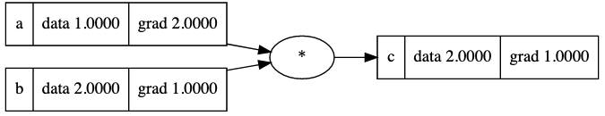
The full operations that are happening here is $\frac{d c}{d c}\frac{\partial c}{\partial a} = 1.0 * b = 2.0$ and $\frac{d c}{d c}\frac{\partial c}{\partial b} = 1.0 * a = 1.0$ , since we are multiplying the “local” gradients of $a$ and $b$ by the downstream gradient, $\frac{dc}{dc} = 1$ . The next computational graph example will make this gradient flow more concrete.

Now that you’ve seen how derivatives are computed on a computational graph, we can apply these to a specific instance of a computational graph - a neural network.

The ultimate goal of a neural network is to make accurate predictions. In order to assess how well the network makes predictions, we consider a loss function, which, given a prediction and a true label, rates how close the network was to being correct. If the network is performing poorly, the loss will be high, and if the network is performing well, the loss will be low. It makes sense that the The final output of the network will be this loss function.

If computing gradients, it’s very important that every operation in a computational graph be differentiable. If an operation is not differentiable, we will not be able to flow the gradient backwards through that node. For example, the absolute value function is non-differentiable at zero, so we would not be able to use it in a computational graph that we are computing gradients for. Since the network is composed entirely of differentiable functions, we can calculate the derivatives of weights at any depth with respect to the loss function.

This gradient computation is really all pytorch and tensorflow are doing, but they are doing it at the level of tensors (i.e. N-D arrays), and they are doing it much more quickly (because it’s parallelized on a GPU).

If you have anything to add, please contact me at will [at] willbeckman [dot] com

Table of Contents